Lorentz' dev blog

This is the first part of my notes on trying to learn machine learning and implementing a simple neural network from scratch in C. The code is intentionally very raw - we don’t even have a function matrix multiplication, I think this makes the details in the algorithms and math stand out more.

The source code can be found here: https://github.com/loldot/nn

Linear regression

An linear function is a function with a single variable whose graph looks like a straight line. We can generalize the function as having a weight \(w\) and a bias \(b\). Changing the weight will change the slope of the line, and changing the bias will change where the line intersects the y-axis. You might remember this equation from high school:

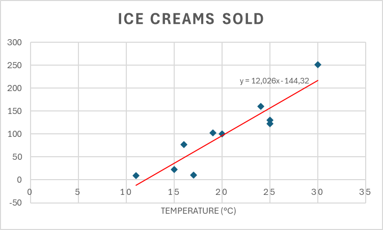
This simple equation can have predictive power if the data fits a line. For example assume we own a small ice cream shop and start measuring the temperature at midday and count our number of ice creams sold. After a few days of measurements, we have the following data:

Our mission is to create a formula that takes the temperature and predicts the number of ice creams sold that day. To approximate this manually, we can choose to points that seem to go somewhere in the middle of the data. Let’s say we choose the data points (15°C, 23) and (30°C, 251). We can then calculate the weight: \(w = \frac{251 - 23}{30 - 15} = 15.2\) This means that if the temperature increases by one degree, we can expect to sell about 15 more ice creams. We can now update our function to \(f(x) = 15.2x + b\). To find a value for \(b\) we can plot the values from our first data point.

Our prediction function is now: \(f(x)= 15.2x - 205\). Now if the weather forecast for tomorrow shows 27°C we can predict that we will sell \(15.2*27 - 205 = 204\) ice creams.

In our manual approximation, we just chose two “good” data points to find our line, and as it turns out, that was pretty hard to do even for a human. There is a better method to find our values for \(w\) and \(b\), called linear regression. Linear regression will find values that minimize the difference between our actual measurements and the line drawn with our weight and bias.

I added a linear regression line to the previous Excel chart, and it appears we were slightly too optimistic with our weight; we can only expect our sales to increase by 12 ice creams when the temperature increases by one - not 15 as we predicted.

Next we will learn a better method to find this line programmatically.

Cost function

Suppose we just guess our initial values for \(w\) and \(b\). Then what we need is a function that can help us determine how well our line fits the data and a function to tell us how we can change \(w\) and \(b\) to improve the fit. A function that measures the difference between our measurements and our prediction is often referred to as the cost function of our model

One way such function is the mean squared error function.

• \(m\) is the total number of observations
• \(y_i\) is the observed number of ice creams sold for data point i
• \(\hat{y}_i\) is the predicted number of ice creams sold for data point i.

// The function we use to predict our number of ice creams sold given a temperature x
// It will become clear later why we call this function "forward"
float forward(float x)
{
    return w * x + b;
}


float cost(const size_t m, const float[m] x, const float[m] y)
{
    float cost = 0.0f;

    for (size_t i = 0; i < m; i++)
    {
        float output = forward(x[i]);
        float error = y[i] - output;

        cost += error * error;
    }

    return cost / m;
}

The question now becomes, how do we reduce the “cost” of our regression line?

Gradient Descent

While there exist many simpler methods to calculate a regression line for such a simple dataset, in the context of machine learning and neural networks, we would rather use a method that is a bit complex, but in the end it will be useful for our neural network later.

To find the optimal regression line, we start by guessing values for \(w\) and \(b\) and calculate the loss function for our data. This will give us a point on a surface like the one showed below. The intuitive explanation for the method we are using is that we will try to take a step in the direction that most quickly moves us towards the bottom of this “bowl”.

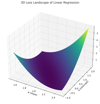
This method is called gradient descent and involves some pretty advanced calculus called partial derivatives to determine direction we have to move.

Before we begin our partial derivatives, we will update our cost function so that it becomes a little easier to work with. Instead of dividing by \(m\), we will divide our mean by two. This small change should not have an effect on our result, but will make the derivatives a little nicer. Now our cost function becomes:

To minimize this cost function, we calculate the partial derivatives with respect to \(w\) and \(b\):

Lets start with the partial derivative with respect to \(w\): \(\frac{\partial}{\partial w} \left( \frac{1}{2m} \sum_{i=1}^m{(y_i-\hat{y}_i)^2} \right)\)

If you think this looks like gobbledygook, you are not alone.

First off, what happened to the \(d\) in \(\frac{d}{dx}\)? The \(\partial\) symbolizes that this is a partial derivative – our cost function has two variables, \(w\) and \(b\), but in this case we only want to understand how \(w\) affects the cost function.

The second question is perhaps how we derive a sum operation? The sum operator is just a shorthand summing all the individual parts of our equation. We could write it as:

Remember that we can differentiate each term in a sum individually, so for now we will just ignore the sum operator and focus on the \((y_i - \hat{y}_i)^2\) part.

First we expand \((y_i - \hat{y}_i)^2\) to \((y_i - (wx_i + b))^2\) using the definition of our forward function.

Let \(e_i=y_i−(wx_i+b)\), we can then apply the chain rule of derivatives:

Note that in the partial derivative, we can consider \(b\) as a constant. We then expand back to: \(\frac{\partial}{\partial w}(y_i - (wx_i + b))^2 = -2(y_i−(wx_i+b)) = -2(y_i−\hat{y_i})x_i\)

We now know how to find the partial derivative of our individual parts of the cost function and can expand the series to

To find the partial derivative with respect to \(b\), we follow the same approach as we did when found the partial derivative with respect to \(w\).

The only difference is the derivative of the inner term:

As before, w let \(e_i=y_i−(wx_i+b)\) when applying the cain rule. When we differentiate with respects to \(b\), \(w\) and \(x_i\) are treated as constants.

These derivatives tell us how to adjust \(w\) and \(b\) to reduce the cost. By iteratively updating \(w\) and \(b\) in the opposite direction of these gradients, we can find the values that minimize the cost function.

void gradient_descent(float x[m], float y[m])
{
    // The number of times we will update the weights and bias is called epochs.
    // The more epochs, the more accurate the model will be.
    const int epochs = 20000;

    // The learning rate (often represented with the greek letter alpha, α) below is 
    // chosen by trial and error to make the function converge faster.

    // In practice this value is usually somewhere between 0.01 and 0.1
    const float learning_rate = 0.1;

    for (size_t e = 0; e < epochs; e++)
    {
        float dw = 0.0f;
        float db = 0.0f;

        for (size_t i = 0; i < m; i++)
        {
            float output = forward(x[i]);

            // Calculate the partial derivatives for w and b.

            // Note: It is common to have the operands the other way around, i.e.
            // error = output - y[i], which will change the sign of the derivative.
            float error = y[i] - output;

            dw += error * x[i];
            db += error;
        }

        dw /= m;
        db /= m;

        w += learning_rate * dw;
        b += learning_rate * db;
    }
}

Continue to part 2